
In May 2008, I had a discussion with Dr. Les Henry from the University of Saskatchewan about EM surveys and soil salinity. It ended with my coming out to the U of S Goodale Farm to conduct an EM survey on a dryland saline seep. I was able to calibrate my GEM2 sensors against his EM38, which in turn, he had calibrated against soil analytical data. Over the next 8 years, I kept coming back to that site to check the calibration of my two conductivity sensors, eventually ending up with almost 50 EM surveys at various times of the year.
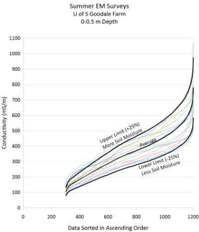
In the winter of 2016, I started looking at the data to see if there was anything else that could be done with it besides just checking the performance of two instruments. I was quite amazed at the variability of EM data when I first graphed the summer data. The range was ±25% from the average. I concluded that most of the variability was due to soil moisture, with data above the average due to times when there was more moisture in the soil and data below the average in drier conditions. The same degree of variability also exists at another site where I have an abundance of data.
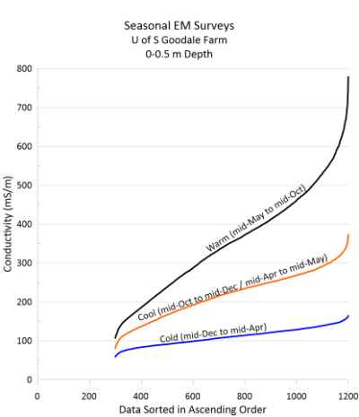
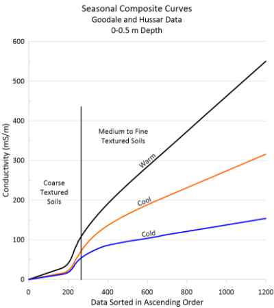
When I started graphing the Goodale Farm data, three distinct groupings were revealed. There was summer or warm season data, roughly mid-May to mid-October, fall/spring or cool season (mid-October to mid-December and mid-April to mid-May) and winter or cold season data (mid-December to mid-April). Although only the surface data are shown here, the curves were similar for the other 4 depths, though the slope of the linear portion of the lines decreased with depth. By the 7m depth, the difference between the warm curve and the cold curve was not nearly as pronounced as at the surface.
At this point, it appeared to be quite feasible to develop a seasonal correction for EM surveys and the algorithms calculated from this data did work very well for some sites, but not at all with other sites. The problem was that the Goodale Farm data started at about 100 mS/m and went up to about 800 mS/m, but the shape of the curve between 100 and zero was unknown. Attempts to simulate the data between 0 and 100 trying various shapes of curves were met with little success and eventually it was concluded that a coarse textured site was needed where real data between 0 and 100 mS/m could be collected.
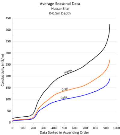
I went through my data from previous EM surveys and found several likely sites that would provide data at the low end. The best site was a combination of proximity to Calgary, year-round access and landowner permission. I ended up with a site near Hussar, AB in native prairie, which had a good gravel road into it. As it turned out, I only compete with the cows for about 6 weeks out of the year. Over the course of 2017 to 2019, I went out to this site about 45 times and collected data from almost 100 surveys. When the data was graphed, there was still a range of about ±25% in the summer data, which appeared to be the influence of soil moisture on the EM survey readings. There were three distinct seasonal groupings and the monthly range was similar to the Goodale Farm data.
At this point, I decided to develop seasonal correction curves for coarse textured soils based on the Hussar data and medium to fine textured soils based on the Goodale Farm data. This approach worked better, but still not with the precision I wanted. One of the biggest drawbacks to having separate sets of curves for coarse and medium to fine textured soils is deciding what the texture of the soil is. Soil survey information across Western Canada is just not detailed enough to determine the texture of the soil from the surface down to 7 m.
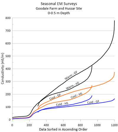
While I did use the two sets of correction curves briefly in 2019, the idea of combining the two data sets occurred to me. As shown in the graph opposite, there appear to be points of inflection between the two data sets where a single curve might be created. I have found that all EM data appears to have the same shape when the data are arranged in ascending order and they do not originate near zero.
Whether from a GEM2 or an EM38/31, the data are exponentially low at the low end and exponentially high at the high end with a long linear slope in the middle. EM data also display different behavior at values close to zero and all sites I have graphed tend to behave like the data from the Hussar site. The curves drop off rapidly to a minimum value and then tend to be linear with a very gradual slope towards zero.
The final composite curve models that arose out of the two data sets preserved as much of the original data from both data sets as was feasible. The low ends of the curves were virtually the Hussar data with little modification, which represented the correction curve for coarse textured soils. The high end of the curves tended to be just the linear portions of the Goodale Farm data, which represented the correction curves for medium and fine textured soils. The high end of the Hussar data was not used as it was found to lie within the range of ±25% for the linear portion of the composite curve.
The models were made to be linear at the high end so as not to overestimate higher conductivities when correcting data from cool or cold seasons to simulate warmer summertime EM surveys.
Early in 2020, I decided I need to test the composite correction curves. I came up with a list of reclaimed sites within a few hours of Calgary and contacted landowners for permission to perform 3 separate surveys on the sites in winter, fall or spring and summer. There were 4 sites in each of the Brown, Dark Brown and Black soil zones and 2 sites in the Dark Grey zone. Of the sites, 6 were coarse textured and the rest were medium to fine textured.
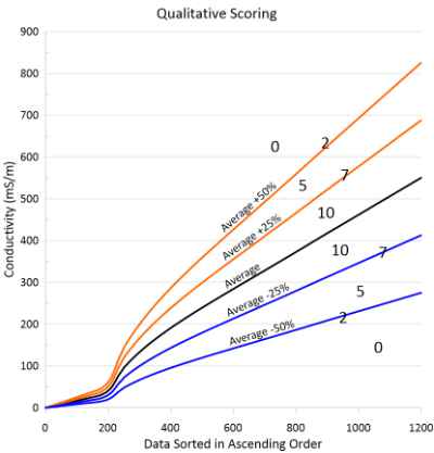
Correlation of the seasonal correction to summertime or warm values was conducted qualitatively by assigning a value of 10 to a corrected curve that lay within the range of ±25% of the warm values. If the corrected curve was mostly at the upper or lower limit, it was given a value of 7 and if it lay outside the range ±25% but inside the range ±50%, it was given a value of 5. If the data was mostly along the 50% line, the assigned value was 2 and outside of 50%, the value was 0. In analyzing results from the 14 sites, none of the data was outside of the 50% interval. The results were strongly biased to soil texture. Medium to fine textured sites averaged 95% agreement from cool season data corrected to warm season and 89% agreement from cold season data corrected to warm seasonal values. For coarse textured soils, there was 89% correlation between cool seasonal data corrected to warm values and 73% correlation for cold season data corrected to warm values.
The reason that cold or winter EM surveys in coarse textured soils did not correct reliably to summertime values is related to soil moisture. The conductivity levels in coarse textured soils are so low, that most of the conductivity at depth is due to existing soil moisture and in the winter this moisture is frozen, resulting in conductivity values near zero. So, the corrected conductivities will still be close to zero throughout most of the conductivity range and will graph below the lower limit (-25%) of the site. When the conductivity values do increase naturally, they get corrected by the exponential portion of the curve and end up above the upper limit (+25%) for the site.
In conclusion, seasonal correction of EM surveys on coarse textured soils in the winter does not appear to be reliable. However seasonal correction of EM surveys conducted on medium and fine textured soils in winter and fall or spring, as well as surveys conducted on coarse textured soils in the fall or spring can be corrected to summertime values with a high degree of reliability.